Analyzing Atlanta's SFR Housing Market

Note: This report is written using markdown, and will reference source code written in the raw.ipynb. I decided to use this format so it’s clearer for the reader, and will provide a .pdf for this report and a .pdf of the source code so you don’t need to go into a .ipynb reader to look at the source code.

Introduction

This report looks to analyze house listings sourced from MLS that were actively listed as of 4/29/2021. We hope to model Atlanta’s SFR (single-family housing) market by comparing different regression models to explore which various factors influence home prices in the Atlanta region, and potentially identify areas that might be good for investment if we can find under-priced homes using our model.

According to this article, we see a rise of interest in investment in the Atlanta region, which makes this analysis relevant to today’s demand.

Listing Prices: Realtor.com’s April 2021 report shows Atlanta is a seller’s real estate market, which means that more people are looking to buy than there are homes available. Home prices have been surging largely because of limited supply and fierce competition for available homes.

The median list price of homes in Atlanta, GA was $379,900, trending up 16.9% year-over-year while the median sale price was $345,500.

Data Exploration:

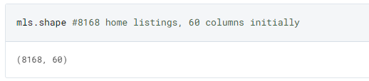
The original data was made up of 8,168 listings, with 23 initial main features + 37 extra features made of arrays of miscellaneous features that only some homes included.

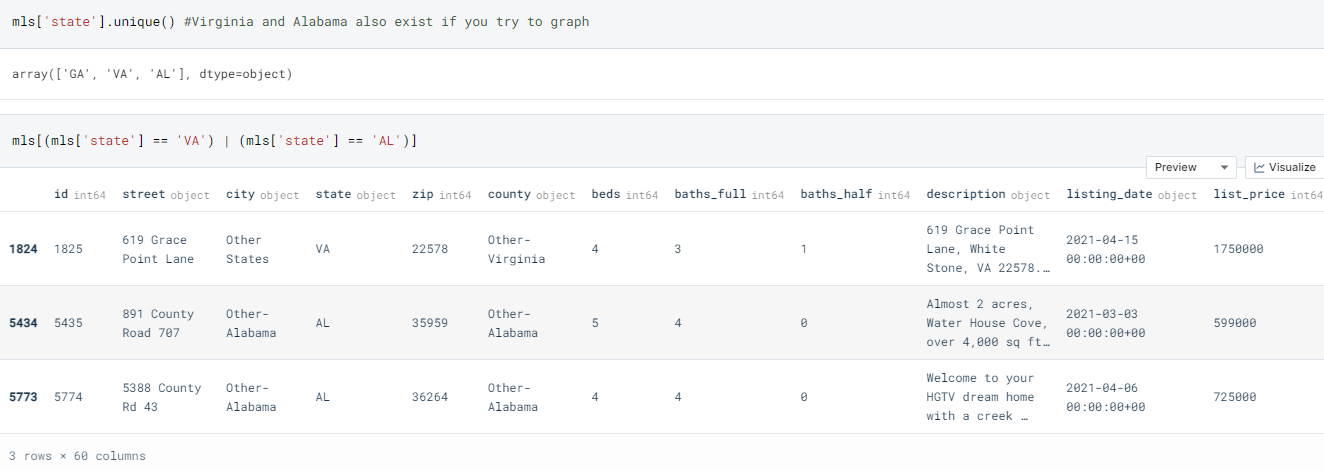
It became immediately obvious that although the report stated that it included only homes in Atlanta, that other cities of Georgia was also included. Additionally, many errors in how (lat,long) was scraped or sourced made it impossible to accurately map coordinates in a local GIS system.

We find that some listings from Virginia and Alabama were included, and were removed for future analysis as we plan to focus on Atlanta.

Below maps the points into a Python package known as Folium; this image shows that current lat/longitude coordinates need to be fixed for some listings.

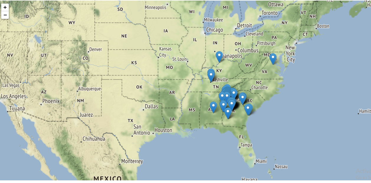
For the sake of time, I will not attempt to map listings to a GIS system to explore trends of house prices and house features among different regions in Atlanta, due to the construction of some parts of the dataset. For an actual analysis, I think understanding the context of different regions in Georgia is important, but given the time constraints (3-5 hours, I rather explore the modeling process more thoroughly). However, since I lack domain knowledge, this is something that might affect later analysis.

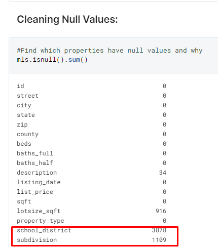
In addition to some coordinates being wrong for some listings, many of the listings have null or no values, particularly for features school district and subdivision:

The picture below only shows a subset of columns with missing values
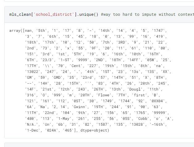
This is hard to impute given the nonsensical way it was coded, and without context it’s best to leave these features out for the analysis (below shows all unique values of school district):
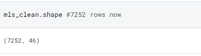
I decided to also drop the 916 listings with null value for lotsize_sqft, as there is no correct value to impute these listings without increasing variance for our future models.
- After removing some redundant features and unusable rows, this leaves us with a starting dataset of 7,252 listings and 46 house features to work with:

Initial Visualization:

Since I do not plan to visualize these listings in a GIS system to infer geographic trends, I still think it’s best to contextualize how well Atlanta’s housing market is to other cities in Georgia.

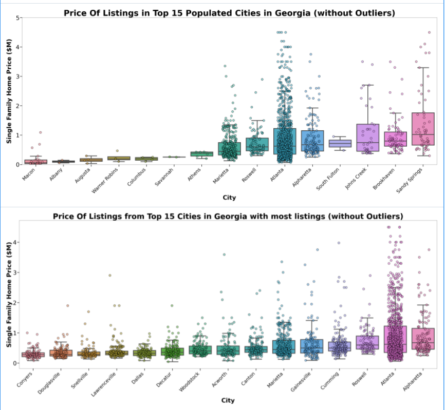
The following boxplots were used using the python package Seaborn where the 15 most populated cities in Georgia were selected as comparison. The graphs also include the 15 cities with the most listings from the dataset, as there might be bias from the lack of data from the other graphs.

Outliers have been removed for visual clarity.

–

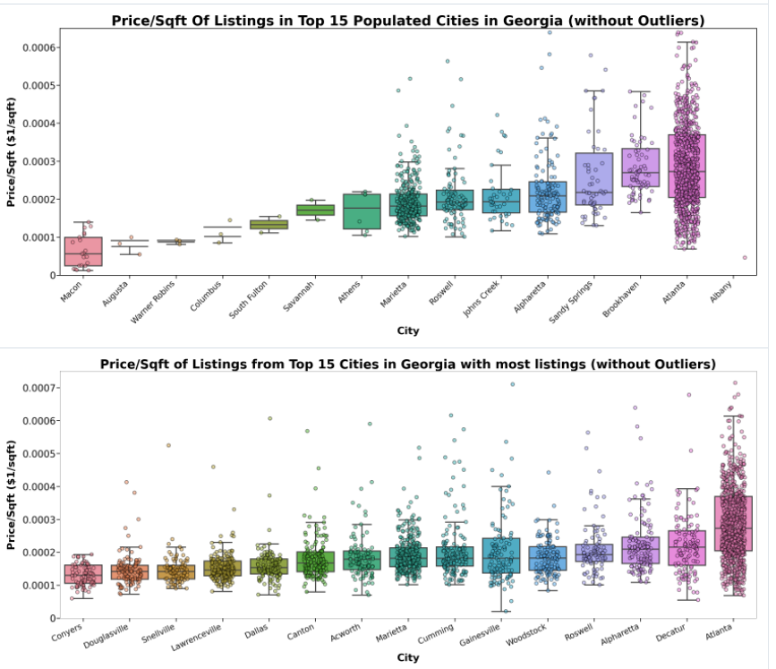
**Analyzing Price Listings: **

As shown below, the cities are ordered based on the median house price-listings from this dataset.

We find that Atlanta has the sixth-highest median compared to the top 15 populated cities in Georgia, and also has the highest peak if we count outliers.
Additionally, we also see that Atlanta has the second highest median out of the top 15 cities with the most listings. However, due to bias that this dataset scraped more Atlanta listings compared to other cities, there may have been a selection bias. Still, we can get a rough estimate of Atlanta’s housing interval through the boxplot, where at least 50% of housings remain between [$500,000, $1,500,000]. Still compared to other cities in Georgia, we find that Atlanta is doing relatively well.

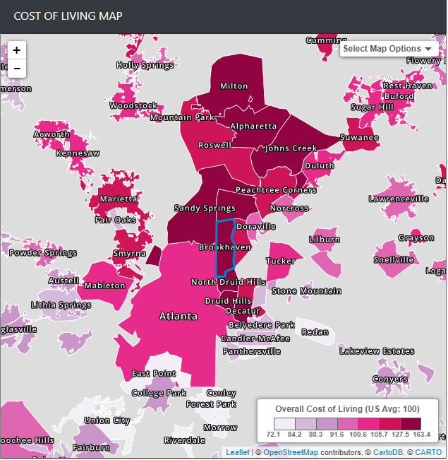
We find that our analysis is rather similar to the actual cost of living of these locations :

source: https://www.bestplaces.net/cost_of_living/city/georgia/brookhaven

Analyzing Lot Price/Sqft

However, in terms of bang-for your buck, it’s quite expensive living in Atlanta. For the amount of lot size you get per sqft, it’s much more expensive to have more space living in Atlanta compared to other cities that are further from living in the capital. Only Brookhaven (which is known to be expensive to live in), and Savannah (which is possibly due to the lack of datapoints) beats Atlanta in the highest median lot price/sqft.

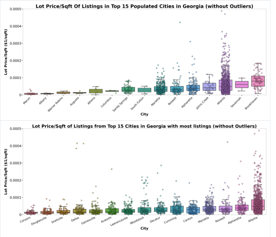
We see a similar conclusion when analyzing listing price/sqft (interior house space). (Excuse the visual bug with Albany)

Modeling:

Given that there seems to be high demand to live near the metropolis given that both Atlanta’s price/sqft and lot price/sqft is the really expensive compared to other cities, we should focus on creating a model to evaluate which features causes this and how we can exploit the model to find under-priced houses to invest in.

We can use a correlation heatmap to initially determine some features that correlate (if there a linear trend between two variables), to contextualize which features may impact list_price. Out of some features from the initial dataset, we find that beds, baths_full, sq_ft, ` baths_full` have the strongest correlations.
Given that we do not plan to use regression, but decision trees for our models, we do not have to worry about multicollinearity from this analysis.

![image-20210620192258593](C:\Users\ferdi\AppData\Roaming\Typora\typora-user-images\image-20210620192258593.png

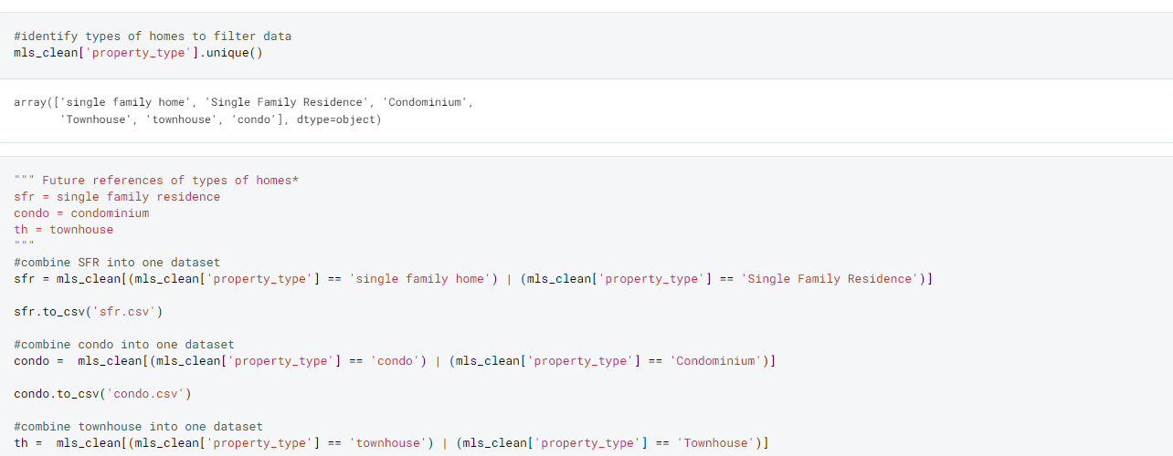
Segmenting the Datasets :

I filtered out any other category homes (townhouses and condos) out of the dataset. I will store these datasets for any future analysis. After including only SFR homes, there are now only 5,916 listings.

Additionally, I filtered homes to only include Atlanta listings, which leaves us with a small sample of 916 listings left to work with for modeling. Given the lack of data-points, I do not expect a model with a strong accuracy for predictions. This is something to be concerned about when actually putting something in production.
For future models, I did a 70/30 training to test split, which caused 642 listings as training data, and 275 listings as test data. Given the lack of data, I did not include another set of validation set to be more precise. If I had more time, I would attempt to use all of Georgia’s dataset to create a general model for the housing market just to use more data points or even scrape more Atlanta listings instead.

Engineering New Features:

I engineered new features based on the features found in the dataset; for the sake of time, I will focus on few in particular, but after everything there are 491 features that was used in the model.

Note: using a lot of new features is very prone to over-fitting for certain models like decision trees, which we will see later in the report.

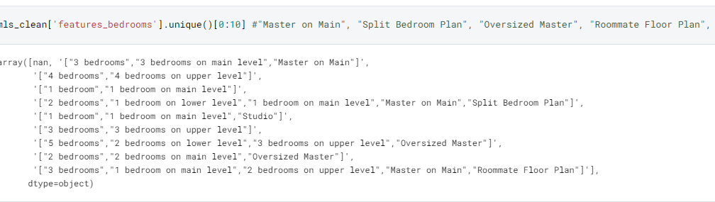
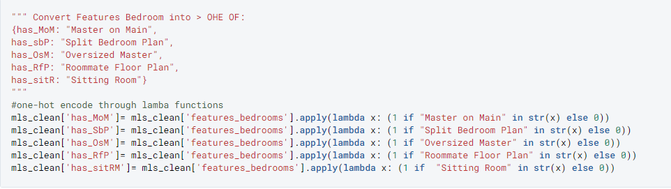
Creating Binary Variables from Features_X: There were 30+ optional features included into the dataset that some homes used, where they included specific features for their household. This included the following:
```
['features_bathrooms', 'features_bedrooms', 'features_dining_room', 'features_fireplaces', 'features_fees', 'features_garage', 'features_heating', 'features_home_owners_association', 'features_house', 'features_interior_features', 'features_kitchen', 'features_laundry', 'features_location', 'features_lot', 'features_parking', 'features_property', 'features_property_access', 'features_roof', 'features_sewer', 'features_taxes', 'features_water', 'features_utilities']
```
- The plan was to engineer new features from the list of feature descriptions. For example, some homes were marked having a “Split Bedroom Plan”, “Oversized Master”, or “Roommate Floor Plan”. I engineered individual binary values to handle these instances. And as a result, 400+ new features were created for future models.

The code format made it easy to modularize for other features:

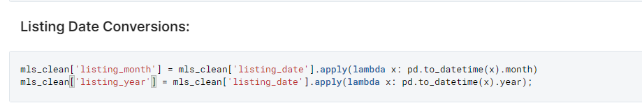
Extract listing month and year: there might be seasonal effects that might affect how listing prices vary over time.
Number of Photos: Some listings might be more detailed with extra information like photos, which might affect the overall listing price. This was pulled from photo_urls

Models:

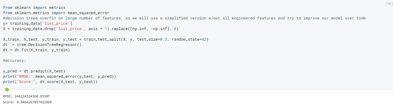
Decision Tree: supervised learning method that can be used to predict listing price, maximizes information gain at each node split (which is powerful when inferring which variables could be important for the model).
- We see that it initially does fairly well (despite RMSE being fairly high however this might be from house listings in the millions). We see that the score of our model is 84% (score is measured by how accurate the predictions are relative to the actual predictions). However, later we see that there was a flaw with this initial model.

However, we see that by looking at the SHAP values (a metric for feature importance in a given model), that I accidently left in heavily correlated variables: price_per_sqft, taxes_in_2020, and lot_price_per_sqft which is scalars of the other two variables.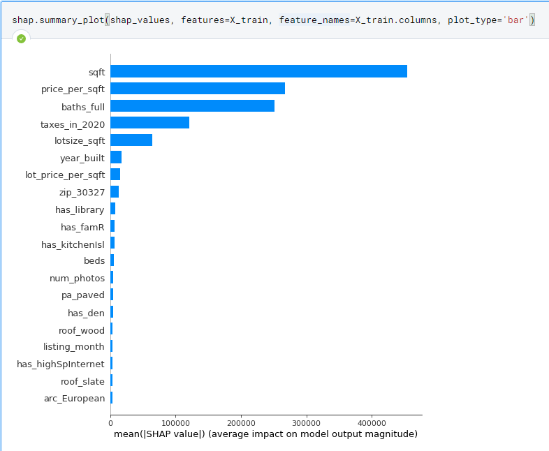
What’s interesting are some of the features that were found to be important for the model like zip_30349, which is an area located south of Atlanta.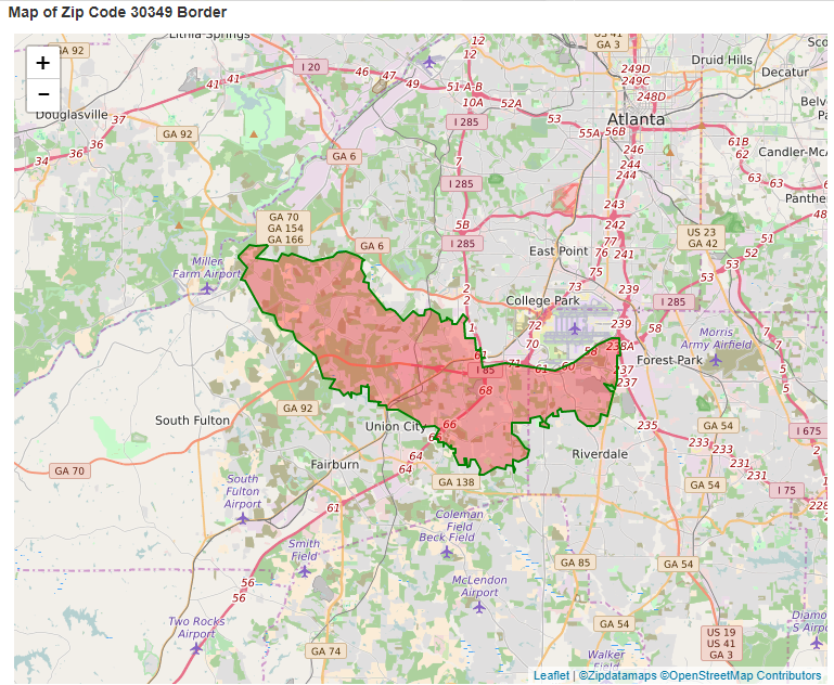
After removing variables that correlate heavily with list_price and limiting the amount of features used to only 15, we still see a decrease in performance for the model:
- Now, the most important features are ones we expected, with some interesting ones now added: num_photos (number of photos in the listing) , roof_composition (if the room is made of composition shingles), has_pantry (if there is a kitchen pantry), has_gasL if there is a gas log for the fireplace, has_famR if there is a family room, and pa_citystr if there is city street parking.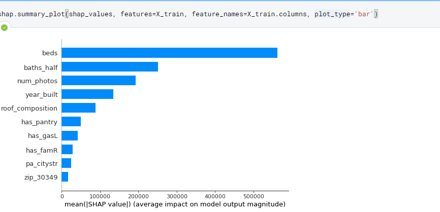

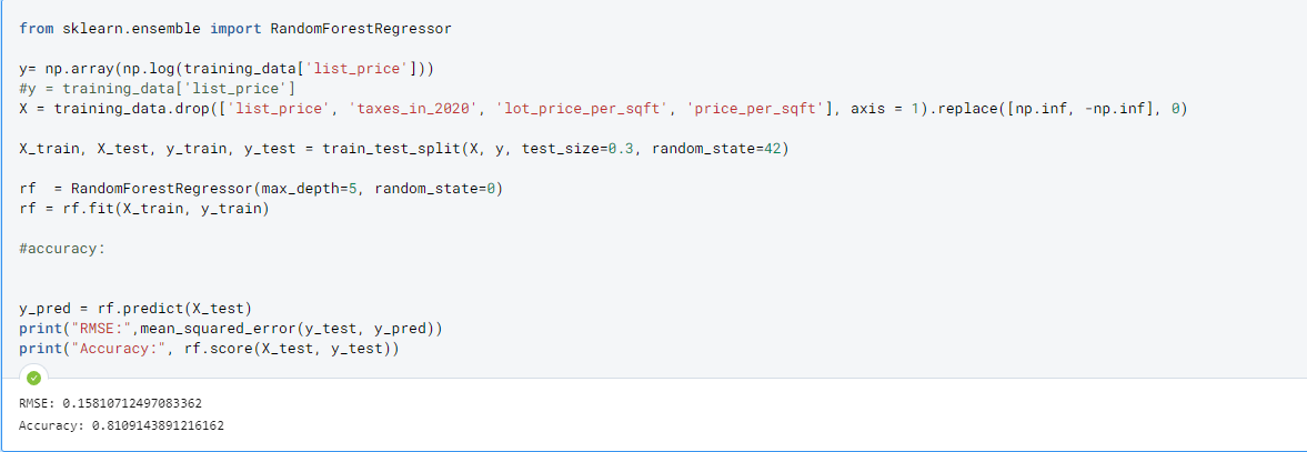
Random Forest: ensemble method bootstrapping multiple decisions trees, and as a result is less prone to over-fitting.
- Another adjustment made to improve performance was to predict the log(listing_price) to increase accuracy, as the scale of predictions was way too large, causing increased variance in predictions. We see that this is a steady improvement from the decision tree model despite removing correlated variables: taxes_in_2020, lot_price_per_sqft, and price_per_sqft.
- We see that performance greatly increased by using Random Forest, with the score boosting up to 81%.

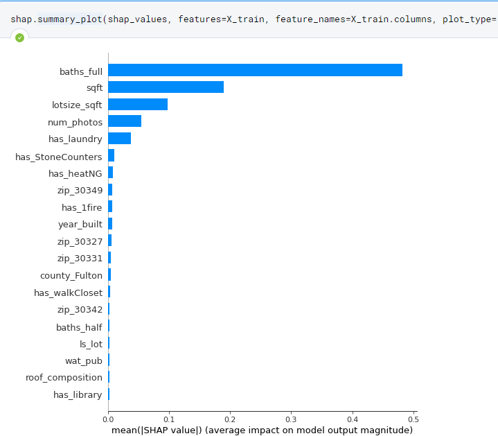
Additionally, the most important features have also changed: with having laundry and having stone kitchen counters as some important features that helped predict listing price.

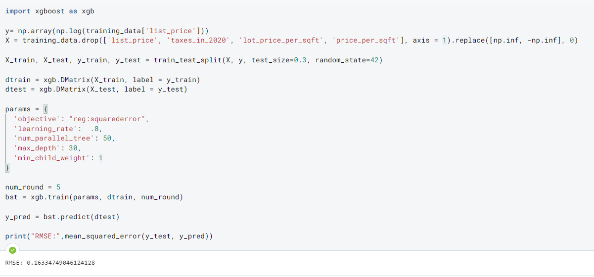
XGBoost: uses gradient boosting instead of bootstrapping of decision trees. One of the best models for maximizing performance.
- Performance slightly increased through the use of XGBoost.
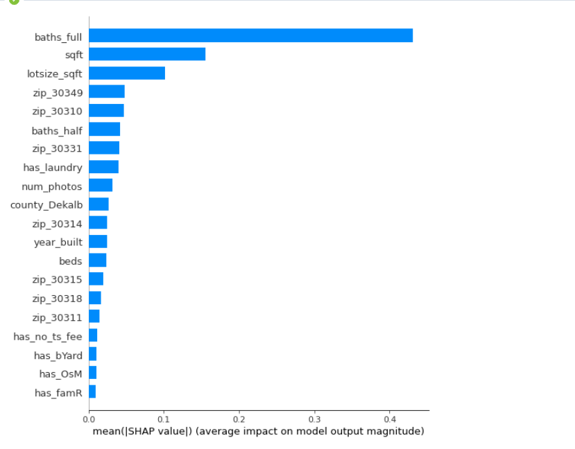
- We see that features surrounding region (zipcode and county) are more important now.

For the interest of my time and making this a concise report, I won’t be exploring how we can use these models for finding under-priced assests.

Conclusion:

Despite the lack of data for the model, we were able to make a decent model that can predict the listing price of future houses in Atlanta. By using this model, we can find current listings and check if it should be priced much higher using our model, a potential way for investors to make profit. Additionally, we now have a general understanding of what features are important in determining house value depending on the model.

What Else To Explore?

The features provided in the dataset provides so much different directions that the project can be improved. Since the accuracy of my model completely failed, there are things that I am missing in my assumptions of the Atlanta housing market. The following are suggestions to improve the quality of the model, or potentially take another route when analyzing the data.
1. Research more about Georgia and Atlanta neighborhoods to understand the unique values of certain features so it can be implemented inside the model.
2. The use of clustering to find segmentation in the housing market (whether it would be by K-means), to include as a feature in our model, or to help house seekers find similar homes that they enjoy using these clusters.
3. The use of NLP to readily process the feature description, whether to engineer new features to improve the model that was not captured by the features that were scraped.
4. Similar to Airbnb, use ML image recognition to identify extra features from photos that could not be captured initially.
5. Scrape and append extra features online that are potential factors to housing prices (like commute times to popular metro hubs or school quality for the nearby district). Since I did not use school district at all, the value of the quality of schools were never captured.
6. Optimize current models based on parameter tuning.