Relearning R

A hodgepodge of notes for learning R for my reference, segmented so it is easy to read.

–

Visualisations

ggplot(data = <DATA>) + 
  <GEOM_FUNCTION>(
     mapping = aes(<MAPPINGS>),
     stat = <STAT>, 
     position = <POSITION>
  ) +
  <COORDINATE_FUNCTION> +
  <FACET_FUNCTION>

Limit axes: + coord_cartesian(ylim = c(0, 50))
- Use xlim for x-axis
use facets: subplots that display subsets of data (categorical variables)

ggplot(data = mpg) + 
  geom_point(mapping = aes(x = displ, y = hwy)) + 
  facet_wrap(~ class, nrow = 2)

also can use facet_grid() to plot combination of two variables:

ggplot(data = mpg) + 
  geom_point(mapping = aes(x = displ, y = hwy)) + 
  facet_grid(drv ~ cyl)

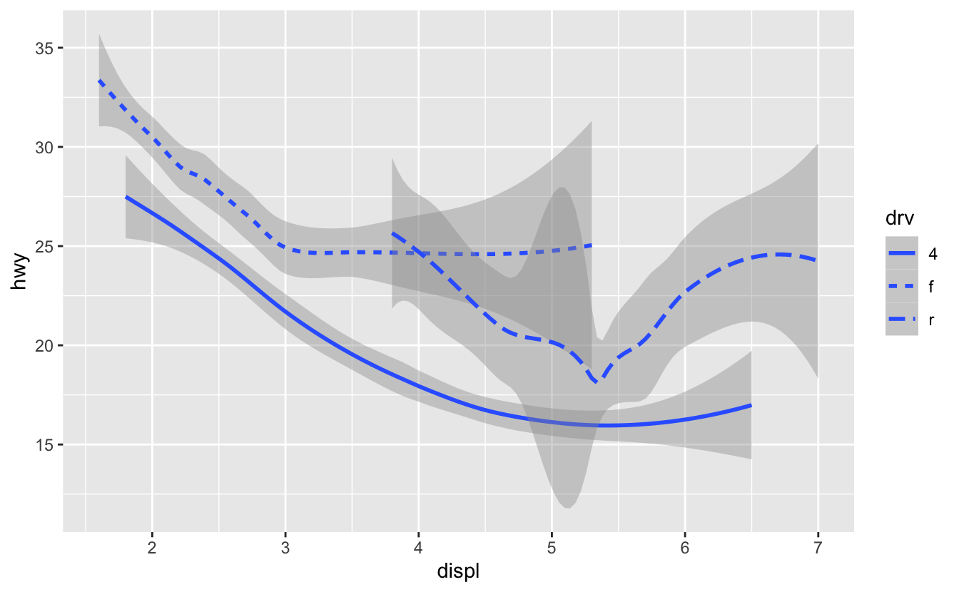
geom_point vs geom_smooth; which object to map plots; every geom function takes mapping as an argument; instead of linetype below, can also use group to show different types of categories with same linetype
```
ggplot(data = mpg) + 
  geom_smooth(mapping = aes(x = displ, y = hwy, linetype = drv))
```

repetition isn’t necessary:

ggplot(data = mpg, mapping = aes(x = displ, y = hwy)) + 
  geom_point(mapping = aes(color = class)) + 
  geom_smooth(data = filter(mpg, class == "subcompact"), se = FALSE)

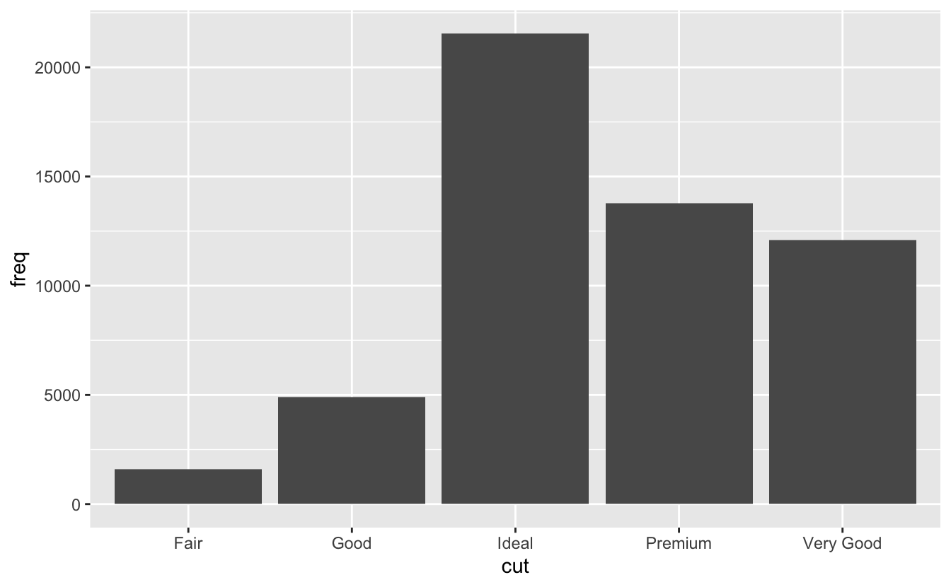
changing order of bar chart for categorical mappings (so doesn’t order based on increasing frequency):

demo <- tribble(
  ~cut,         ~freq,
  "Fair",       1610,
  "Good",       4906,
  "Very Good",  12082,
  "Premium",    13791,
  "Ideal",      21551
)
  
ggplot(data = demo) +
  geom_bar(mapping = aes(x = cut, y = freq), stat = "identity"
  #use  y = stat(prop) for proportion

lineplots (w stats)/ boxplots:

ggplot(data = diamonds) + 
  stat_summary(
    mapping = aes(x = cut, y = depth),
    fun.min = min,
    fun.max = max,
    fun = median
  )
  
  ggplot(data = mpg, mapping = aes(x = class, y = hwy)) + 
  geom_boxplot() 
  #add + coord_flip() to make it horizontal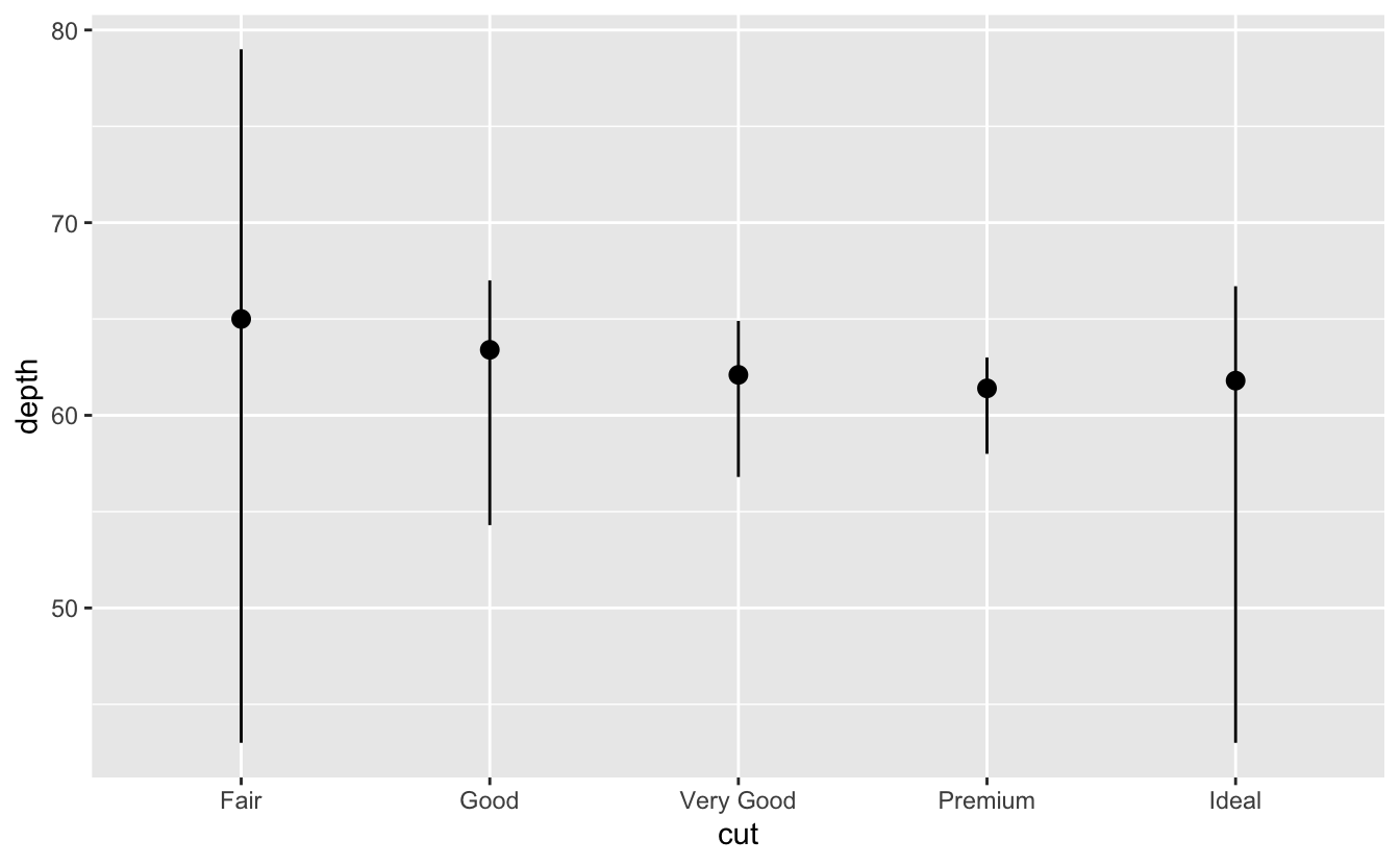

Use reorder to reorder boxplots (FUN is function to use)

ggplot(data = mpg) 
	+ geom_boxplot(mapping = aes(x = reorder(class, hwy, FUN = median), y = hwy)) 

can use fill (also for categorical) to fill whole bars, or normal color for outlines
+ coord_flip() flips the axis

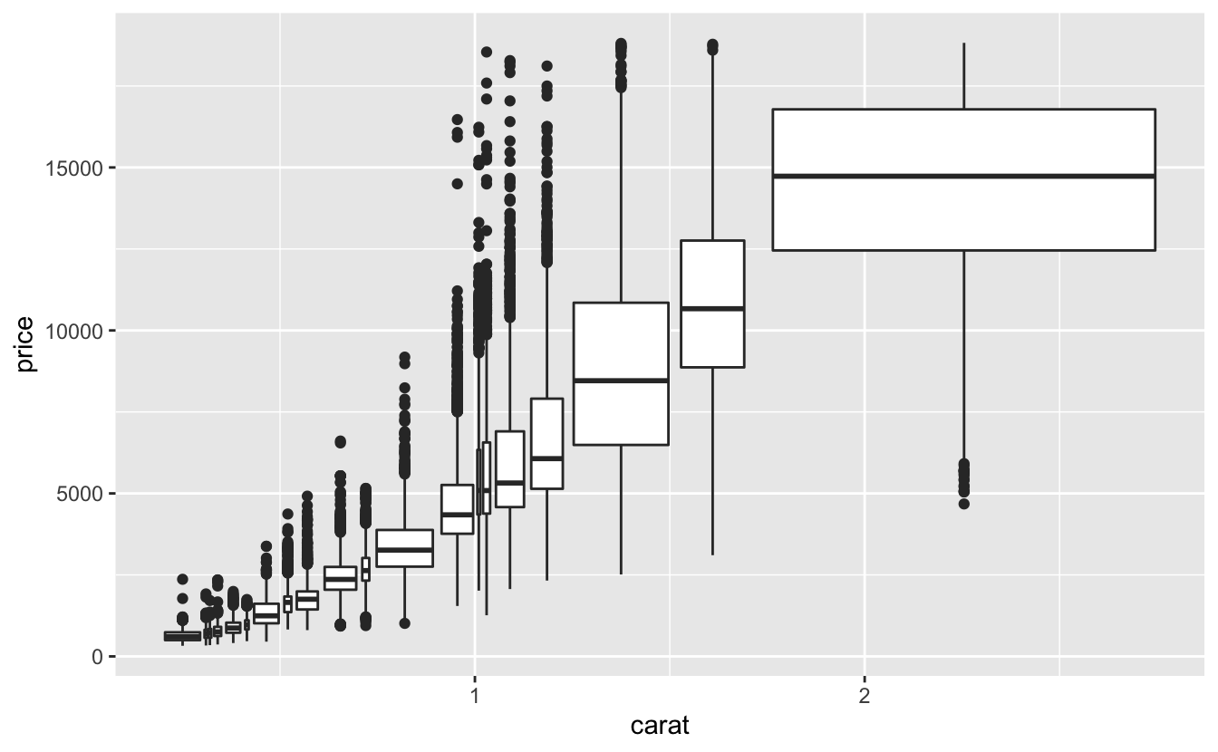
Different boxplot width based on # of points in each bin:

ggplot(data = smaller, mapping = aes(x = carat, y = price)) + 
  geom_boxplot(mapping = aes(group = cut_number(carat, 20)))

position = "identity" will place each object exactly where it falls in the context of the graph. This is not very useful for bars, because it overlaps them. To see that overlapping we either need to make the bars slightly transparent by setting alpha to a small value, or completely transparent by setting fill = NA; basically doesn’t stack like fill, but overlaps on top of each other to see original value compared to y
position = "fill" works like stacking, but makes each set of stacked bars the same height. This makes it easier to compare proportions across groups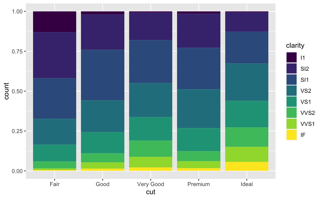
position = "dodge" places overlapping objects directly beside one another. This makes it easier to compare individual values; below image shows this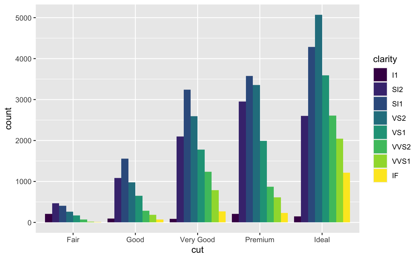
use position = jitter for scatterplot when points over plot with each other; + geom_jitter()
can use bar + coord_polar() to make bar charts into pie charts
explore labs for tags/titles/etc

Instead of using geom_histogram use geom_freqpoly for categories of data:

ggplot(diamonds, aes(price, colour = cut)) 
  + geom_freqpoly(binwidth = 500)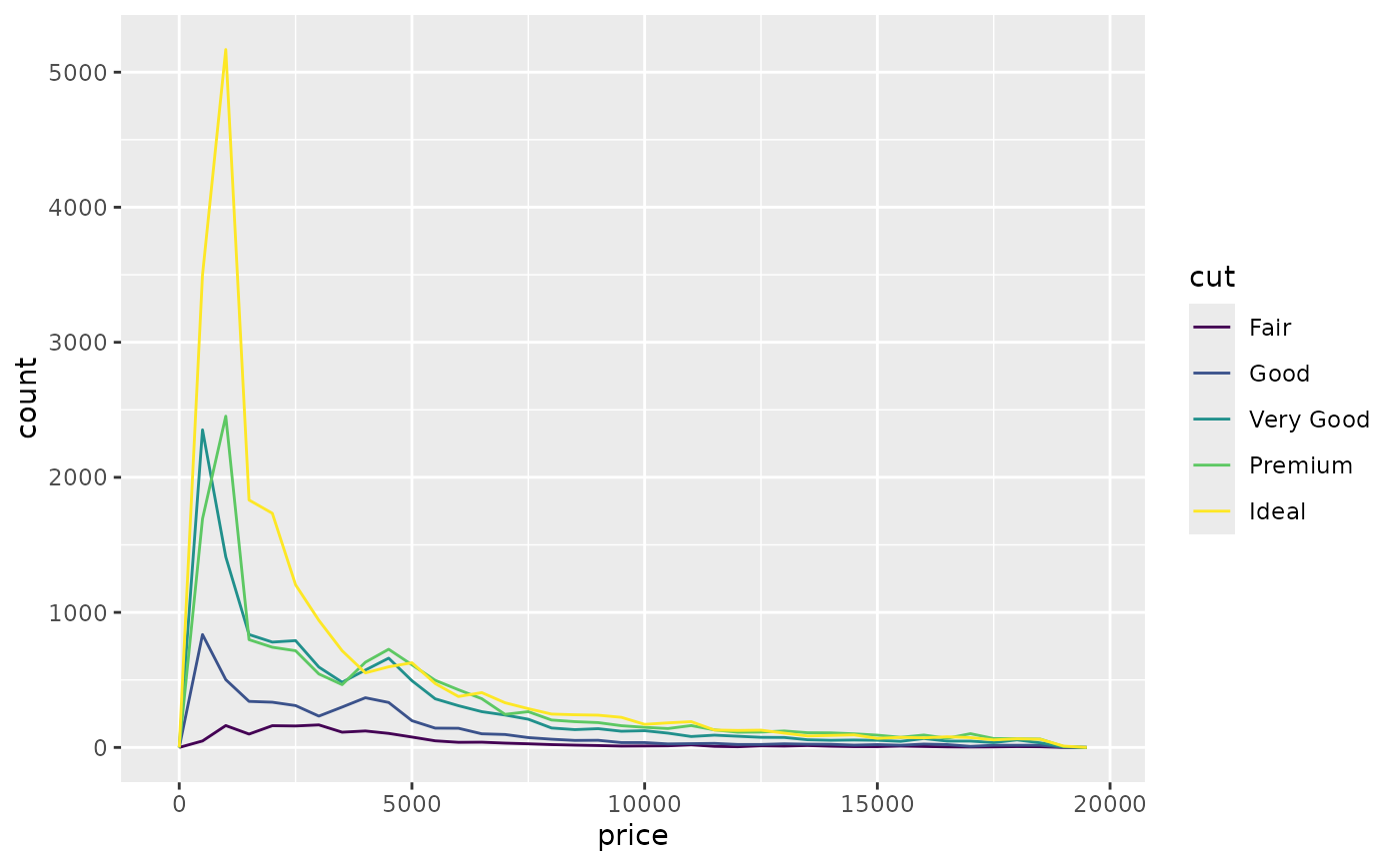

–

The Basics

Do not use =, instead do ALT + - to create <- to assign variables
Use snake case for styling convention (underscore to separate lowercase):

example: i_use_snake_case
Use CTRL + UP_ARROW to look at all commands executed in terminal (fast-ease to re-do past commands)
Variables are case-sensitive – typos will happen
When shifting through different functions using TAB autofill, press F1 to get more detailed documentation
ALT + SHIFT + K to access all keyboard shortcuts
Press Ctrl + Shift + F10 to restart RStudio
Press Ctrl + Shift + S to rerun the current script
dplyr overwrites base functions of R – to access original, use: stats::function
Easy access of functions / objects using ::

one example: nycflights13::flights to access dataframe

To print and save assignments, wrap in parentheses:
- example: (dec25 <- filter(flights, month == 12, day == 25))

When using == to check for boolean conditions, use near instead:

sqrt(2) ^ 2 == 2
#> [1] FALSE
1 / 49 * 49 == 1
#> [1] FALSE
--
near(sqrt(2) ^ 2,  2)
#> [1] TRUE
near(1 / 49 * 49, 1)
#> [1] TRUE

Ctrl + Shift + P to resend the complete block that was recently used in console– useful when editing a block constantly.

Data Transformation

tibbles are dataframes but tweaked to work under tidyverse

vectors can be named (used for subsetting):

c(x = 1, y = 2, z = 4)
#or
set_names(1:3, c("a", "b", "c"))
#> a b c 
#> 1 2 3

subsetting starts at index 1:

x <- c("one", "two", "three", "four", "five")
x[c(3, 2, 5)]
#> [1] "three" "two"   "five"

negative values drop element, and mixing negative and positive do not work:

x[c(-1, -3, -5)]
#> [1] "two"  "four"
x[c(1, -1)]
#> Error in x[c(1, -1)]: only 0's may be mixed with negative subscripts

subsetting in lists with [] returns smaller list, [[]] gets element:

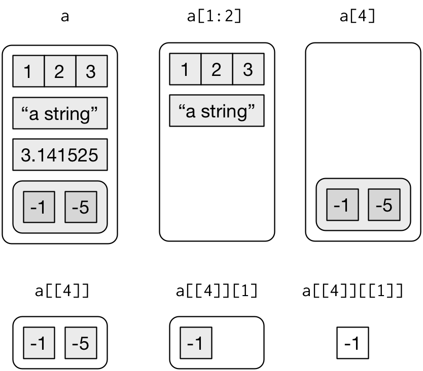
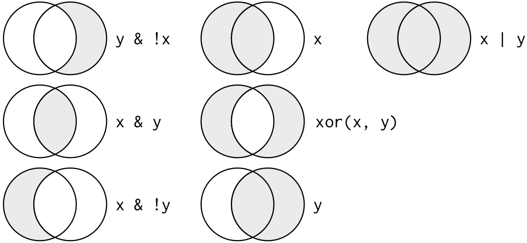
& = “and”, | = “or”, ! = “not”
- Boolean operations in picture:
the following abbreviations for types of variables:
- int: integer, dbl: doubles/real numbers
- chr: character vectors, or strings
- dttm: date-times (date+time)
- lgl: logical (booleans), vectors with only TRUE or FALSE
- fctr: factors (used to represent categorical variables with fixed possible values)

–

the basics of dplyr, in which the first argument is a df:
- Pick observations by their values filter().
  - example:
    filter(flights, !(arr_delay > 120 | dep_delay > 120)) filter(flights, arr_delay <= 120, dep_delay <= 120) #Demorgans law: !(x & y) is the same as !x | !y, #and !(x | y) is the same as !x & !y
  - can use between(x, left, right)instead of boolean condition statements: ` x >= left & x <= right`
- Reorder the rows: arrange()
  - selects rows in ascending order, can use desc() to re-order in descending order: arrange(flights, desc(dep_delay))
- Pick variables by their names: select().
  - Can select columns between two variables: select(flights, year:day)
  - Can select columns not between two variables (inclusive): select(flights, -(year:day))
  - Some helper functions, see ?select for more:
    - starts_with("abc")
    - ends_with("xyz")
    - contains("ijk")
    - everything() pulls all the other variables to re-order
      - num_range("x", 1:3) matches variables x1 to x3
  - Use rename to keep all variables not mentioned (as select drops it)
    - rename(flights, tail_num = tailnum)
- Create new variables with functions of existing variables: mutate().
  - similar to apply() from python; can also refer to columns that you’ve created in the same line; ONLY TEMPORARY unless stored
  - function must be vectorized: it must take a vector of values as input, return a vector with the same number of values as output.
  - adds new variable to end of dataset; use View(df) to see all columns
  - Example:
    flights_sml <- select(flights, year:day, ends_with("delay"), distance, air_time ) mutate(flights_sml, gain = dep_delay - arr_delay, speed = distance / air_time * 60 ) #> # A tibble: 336,776 x 9 #> year month day dep_delay arr_delay distance air_time gain speed #> <int> <int> <int> <dbl> <dbl> <dbl> <dbl> <dbl> <dbl> #> 1 2013 1 1 2 11 1400 227 -9 370.
  - if you only want to keep the new variables, use transmute()
  - %/% = integer division, dividing and then rounding down to nearest integer
  - %% = mod, or just remainder
  - Other functions: lead(), lag() (refers to the number that leads them or is behind them), cumsum(), cumprod(), cummin(), cummax(), cummean()
  - Also ranking functions: min_rank(), row_number(), dense_rank(), percent_rank(), cume_dist(), ntile()
    transmute(flights, dep_time, hour = dep_time %/% 100, minute = dep_time %% 100 ) #> # A tibble: 336,776 x 3 #> dep_time hour minute #> <int> <dbl> <dbl> #> 1 517 5 17 #> 2 533 5 33 #> 3 542 5 42 #> 4 544 5 44 #> 5 554 5 54 #> 6 554 5 54 #> # … with 336,770 more rows
- Collapse many values down to a single summary: summarise().
  - use in tandem with group_by to compute unit of analysis from complete dataset to individual groups.
  - count = n() as a sub function to calculate # of data points
    - sum(!is.na(x)) as a sub function to calculate # of missing values
    - n_distinct(x) for distinct values
  - or can calculate statistics of overall data-frame like mean: summarise(flights, delay = mean(dep_delay, na.rm = TRUE))
- And then can operate by groups: group_by().
  - use ungroup() to ungroup back to one layer
  - also use filters and mutations on groups
- **Piping: ** %>% or read as “then,” which combines all transformations into one code block and it’s easier to read:
  - sequential: x %>% f(y) turns into f(x, y), and x %>% f(y) %>% g(z) turns into g(f(x, y), z) and so on
```
by_dest <- group_by(flights, dest)
delay <- summarise(by_dest,
  count = n(),
  dist = mean(distance, na.rm = TRUE),
  delay = mean(arr_delay, na.rm = TRUE)
)
#> `summarise()` ungrouping output (override with `.groups` argument)
delay <- filter(delay, count > 20, dest != "HNL")
    
## VS. Piping way
    
delays <- flights %>% 
  group_by(dest) %>% 
  summarise(
    count = n(),
    dist = mean(distance, na.rm = TRUE),
    delay = mean(arr_delay, na.rm = TRUE)
  ) %>% 
  filter(count > 20, dest != "HNL")
```
- sum of one variable (total # of miles a certain plane flew), where wt refers to weight of the variable being counted.
  - think of this as a sum of a variable based on another variable
```
not_cancelled %>% 
  count(tailnum, wt = distance)
#> # A tibble: 4,037 x 2
#>   tailnum      n
#>   <chr>    <dbl>
#> 1 D942DN    3418
#> 2 N0EGMQ  239143
#> 3 N10156  109664
#> 4 N102UW   25722
#> 5 N103US   24619
#> 6 N104UW   24616
#> # … with 4,031 more rows
```

Handling Missing Values

NA represents unknown values, and any operations involving will also be unknown
- NA == NA will result in NA given this same premise
- use is.na(x) to determine if value is missing
- can be persevered when filtering:
```
filter(df, is.na(x) | x > 1)
```
- When working with arrange(), missing values will always be sorted at the end, use indicators to have them at the beginning: arrange(flights, desc(is.na(dep_time)), dep_time)

–

Data Exploration/Transformation

Questions to Explore:

Which values are the most common? Why?
Which values are rare? Why? Does that match your expectations?
Can you see any unusual patterns? What might explain them?

Change certain values of column through boolean condition:
```
diamonds2 <- diamonds %>% 
	mutate(y = ifelse(y < 3 | y > 20, NA, y))
```
- Change y: if it meets condition then NA, else y;
- Look into case_when() to create a new variable that does complex combinations of existing variables
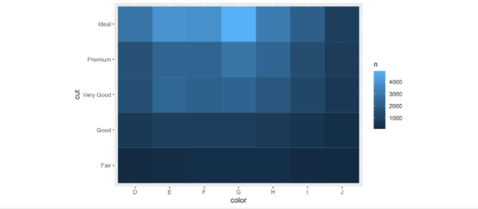
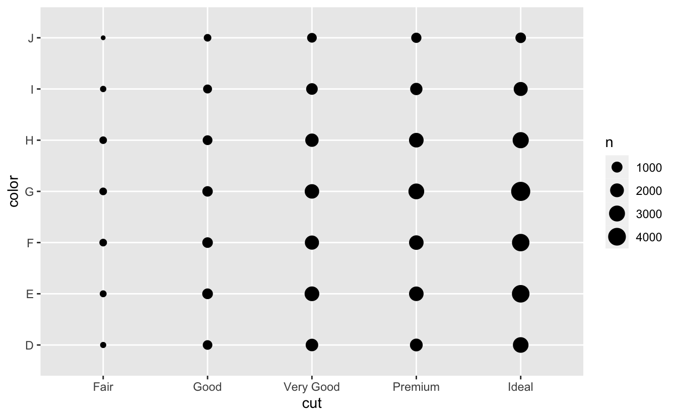
Two ways to visualize covariation with categorical variables:

diamonds %>% count(color, cut) %>% ggplot(mapping = aes(x = color, y = cut)) + geom_tile(mapping = aes(fill = n))

ggplot(data = diamonds) +
  geom_count(mapping = aes(x = cut, y = color))

Using map instead of for loops:

map() makes a list.
map_lgl() makes a logical vector.
map_int() makes an integer vector.
map_dbl() makes a double vector.
map_chr() makes a character vector.

–

Tibbles:

Convert df to tibbles: as_tibble(df)
Convert vector to tibbles: tibble( x = 1:5, y = 1, z = x ^ 2 + y)
- variables x,y,z as functions

Use ` (backticks) to use non-synaptic names

tb <- tibble(
 `:)` = "smile", 
 ` ` = "space",
 `2000` = "number")

Tribbles, create tibbles using tables directly:

  tribble(
    ~x, ~y, ~z,
    #--|--|----
    "a", 2, 3.6,
    "b", 1, 8.5
  )

Different with printing and subsetting (shows only the first 10 rows, and all the columns that fit on screen, each column reports its type, a nice feature borrowed from str
[[can extract by name or position; $only extracts by name but is a little less typing
- tibbles can’t do partial matching
Can convert back to df: class(as.data.frame(tb)) #tb is tibbles

–

Importing and Reading Data (using readrof tidyverse):

read_csv() reads comma delimited files or inline csv files, read_csv2() reads semicolon separated files, read_tsv() reads tab delimited files, and read_delim() reads in files with any delimiter.

a.) na: this specifies the value (or values) that are used to represent missing values in your file

b.) the data might not have column names. you can use col_names = FALSE to tell read_csv() not to treat the first row as headings, and instead label them sequentially from X1 to Xn; alternatively you can pass col_names a character vector which will be used as the column names

c.) sometimes there are a few lines of metadata at the top of the file: use skip = n to skip the first n lines; use comment = "#" to drop all lines that start with (e.g.) #
read_fwf() reads fixed width files. You can specify fields either by their widths with fwf_widths() or their position with fwf_positions()

a) read_table() reads a common variation of fixed width files where columns are separated by white space.
read_log() reads Apache style log files
First argument is the path
Compared to base R, tidyverse creates tibbles and doesn’t convert character vectors to factors

–

Parsing Data:

Like all functions in the tidyverse, the parse_*() functions are uniform: the first argument is a character vector to parse, and the na argument specifies which strings should be treated as missing
- parse_logical() and parse_integer() parse logicals and integers respectively. There’s basically nothing that can go wrong with these parsers so I won’t describe them here further
- parse_double() is a strict numeric parser, and parse_number() is a flexible numeric parser. These are more complicated than you might expect because different parts of the world write numbers in different ways
- parse_character() seems so simple that it shouldn’t be necessary. But one complication makes it quite important: character encodings
- parse_factor() create factors, the data structure that R uses to represent categorical variables with fixed and known values
- parse_datetime(), parse_date(), and parse_time() allow you to parse various date & time specifications. These are the most complicated because there are so many different ways of writing dates
- readr has the notion of a “locale”, an object that specifies parsing options that differ from place to place. When parsing numbers, the most important option is the character you use for the decimal mark. You can override the default value of
- parse_number() addresses the second problem: it ignores non-numeric characters before and after the number
- you need to specify the encoding in parse_character(): parse_character(x1, locale = locale(encoding = “Latin1”)); use guess_encoding() to help you figure it out
- readr also comes with two useful functions for writing data back to disk: write_csv() and write_tsv()
- Every parse_xyz() function has a corresponding col_xyz() function. You use parse_xyz() when the data is in a character vector in R already; you use col_xyz() when you want to tell readr how to load the data.
Example:
```
challenge <- read_csv(
  readr_example("challenge.csv"), 
  col_types = cols(
    x = col_double(),
    y = col_date() ))
  
#Sometimes it’s easier to diagnose problems if you just read in all the columns as character vectors:
challenge2 <- read_csv(readr_example("challenge.csv"), 
  col_types = cols(.default = col_character())
)
```
Custom Date-Time Format Parsing:
Year:
- %Y (4 digits).
- %y (2 digits); 00-69 -> 2000-2069, 70-99 -> 1970-1999.
Month:
- %m (2 digits).
- %b (abbreviated name, like “Jan”).
- %B (full name, “January”).
Day:
- %d (2 digits).
- %e (optional leading space).
Time:
- %H 0-23 hour.
  - %M minutes; %S integer seconds%OS real seconds.
- %I 0-12, must be used with %p.
- %p AM/PM indicator.
- %Z Time zone (as name, e.g. America/Chicago). Beware of abbreviations: if you’re American, note that “EST” is a Canadian time zone that does not have daylight savings time. It is not Eastern Standard Time.
- %z (as offset from UTC, e.g. +0800).
Non-digits:
- %. skips one non-digit character.
- %* skips any number of non-digits.

–

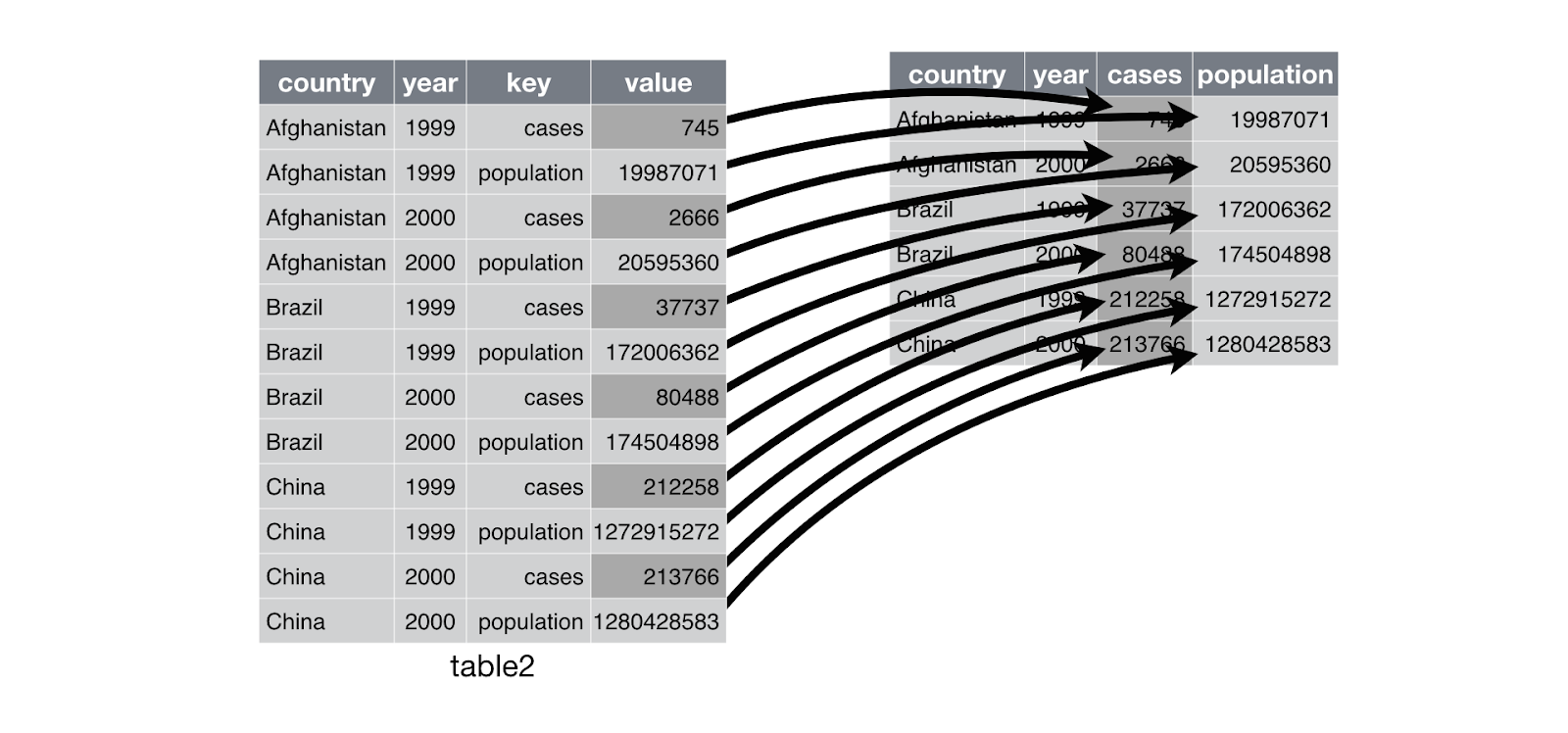
Tidy Data:

Each variable must have its own column.
Each observation must have its own row.
Each value must have its own cell.

There’s a specific advantage to placing variables in columns because it allows R’s vectorised nature to shine. As you learned in mutate and summary functions, most built-in R functions work with vectors of values. That makes transforming tidy data feel particularly natural.

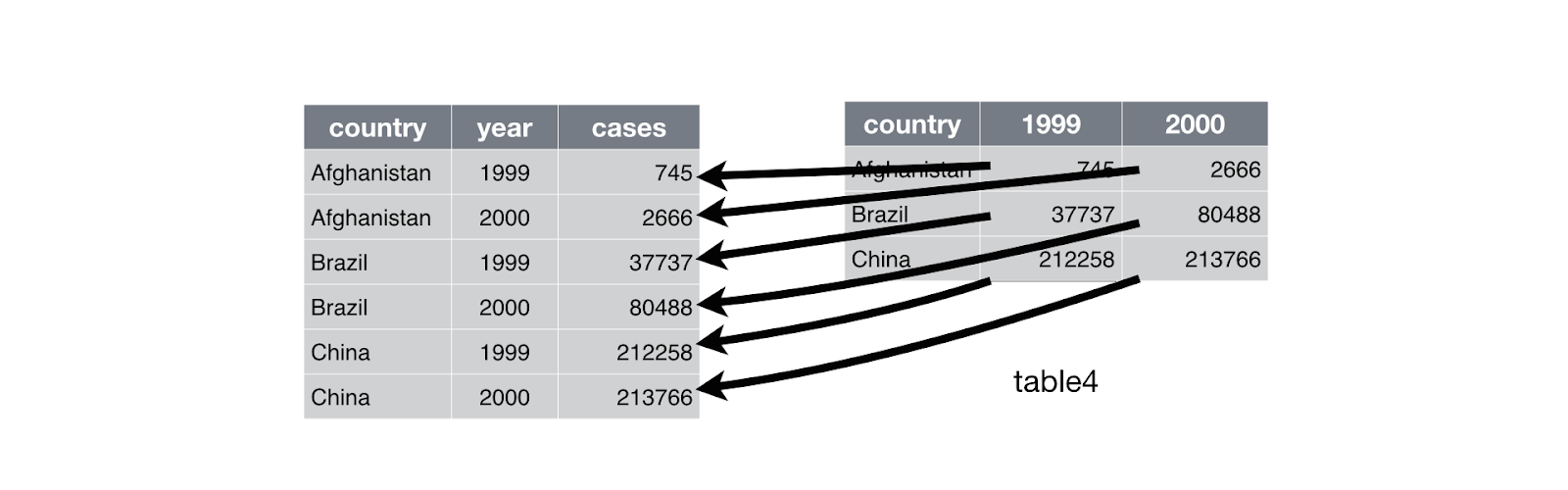
pivot_longer: change observations into columns

table4a
#> # A tibble: 3 x 3
#>   country     `1999` `2000`
#> * <chr>        <int>  <int>
#> 1 Afghanistan    745   2666
#> 2 Brazil       37737  80488
#> 3 China       212258 213766
   
 table4a %>% 
  pivot_longer(c(`1999`, `2000`), names_to = "year", values_to = "cases")
#> # A tibble: 6 x 3
#>   country     year   cases
#>   <chr>       <chr>  <int>
#> 1 Afghanistan 1999     745
#> 2 Afghanistan 2000    2666
#> 3 Brazil      1999   37737
#> 4 Brazil      2000   80488
#> 5 China       1999  212258
#> 6 China       2000  213766
  

Similar to pivot_wider:

–

Memory:

pryr::object_size() gives the memory occupied by all of its arguments.

If two dataframes share the same columns from mutations, etc. then they have the same memory; if one value of one dataframe is changed, then memory is increased since column can no longe rbe shared

–

When to not pipe (%>%)

The pipe is a powerful tool, but it’s not the only tool at your disposal, and it doesn’t solve every problem! Pipes are most useful for rewriting a fairly short linear sequence of operations. I think you should reach for another tool when:

Your pipes are longer than (say) ten steps. In that case, create intermediate objects with meaningful names. That will make debugging easier, because you can more easily check the intermediate results, and it makes it easier to understand your code, because the variable names can help communicate intent.
You have multiple inputs or outputs. If there isn’t one primary object being transformed, but two or more objects being combined together, don’t use the pipe.
You are starting to think about a directed graph with a complex dependency structure. Pipes are fundamentally linear and expressing complex relationships with them will typically yield confusing code.

–

Coercion:

converting one variable type to another

Explicit coercion happens when you call a function like as.logical(), as.integer(), as.double(), or as.character()
- should always try to upstream the change first so the vector isn’t read wrong in the first place (tweak readr col_types)
Implicit coercion happens when you use a vector in a specific context that expects a certain type of vector. For example, when you use a logical vector with a numeric summary function, or when you use a double vector where an integer vector is expected.

Most complex variables of a vector wins for the type of the list:

typeof(c(TRUE, 1L))
#> [1] "integer"
typeof(c(1L, 1.5))
#> [1] "double"
typeof(c(1.5, "a"))
#> [1] "character"

Use the following instead of general is_vector:

	lgl	int	dbl	chr	list
`is_logical()`	x
`is_integer()`		x
`is_double()`			x
`is_numeric()`		x	x
`is_character()`				x
`is_atomic()`	x	x	x	x
`is_list()`					x
`is_vector()`	x	x	x	x	x

–

For more resources:

Notes taken from an online book here